The LabVIEW interface is used for acquiring Fermi surfaces and allows for the automated control of the sample manipulator. The Scienta-Omicron software SES can also be used for measurements at a fixed position in space.

NOTE: Before opening LabVIEW ensure that SES is closed. This can be checked by opening up 'Task Manager' and force quitting any running SES processes. Sometimes this is also necessary to do when leaving LabVIEW to run SES. In this case, close any running LabVIEW processes, before opening SES or you will get an error.

Opening LabVIEW

The acquisition can be accessed with the desktop shortcut labelled: AcquisitionControl_j

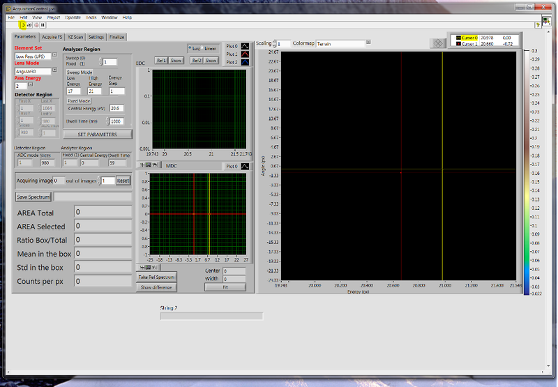
LabVIEW will load giving the following graphical user interface (GUI):

CAUTION: Ensure the last gate valve to the endstation is closed before running the LabVIEW program. This is to ensure that the central energy is at the correct value preventing the analyzer MCP from overloading with counts.

The LabVIEW program starts running by clicking on the 'Run' icon in the top left of the GUI, that looks like a white arrow (highlighted in yellow in the above image). You will then be asked if the system is set up in 'Low Pass' or 'High Pass' mode.

CAUTION: Please confirm that the high voltage cables on the front of the Scienta power supply will match the mode you select in LabVIEW.

If a successful connection has been made with the Scienta analyzer, a live 'Camera Image' window will open up on the monitor as shown below.

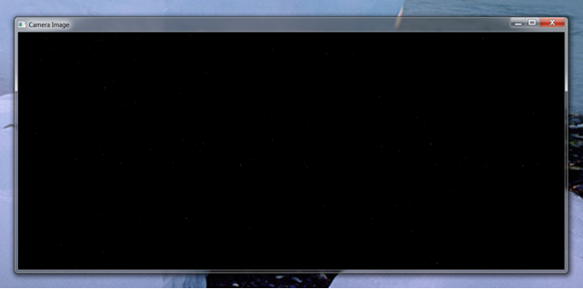
You will not see many 'counts' on the camera image until the last gate valve is reopened.

Parameters such as lens mode, pass energy, kinetic energy, swept/fixed mode, dwell time can all be set in the main display under the 'Parameters' tab.

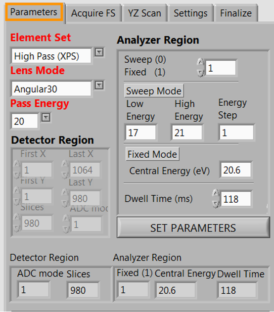
NOTE: some parameters require the 'SET PARAMETERS' button to be clicked before they are registered. It is best practice to click 'SET PARAMETERS' after changing any of the values in 'Element Set', 'Lens Mode', or 'Analyzer Region'. Current settings are in the areas labeled 'Detector Region' and 'Analyzer Region'

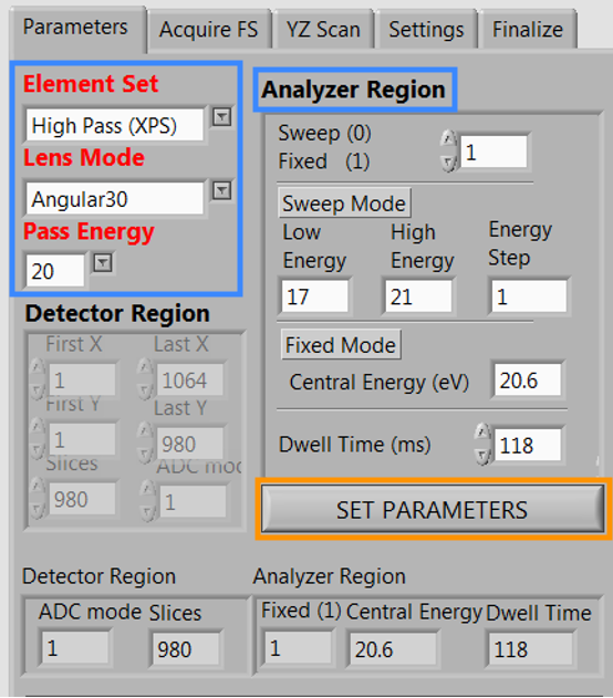
TROUBLESHOOTING: if the 'Detector Region' and 'Analyzer Region' do not reflect your requested values after entry and clicking 'SET PARAMETERS', there is likely a communication error between LabVIEW and the Scienta analyzer power supply. Please close and restart LabVIEW if this occurs. This error often occurs if the Scienta software SES was not properly exited prior to opening the LabVIEW acquisition program.

Parameter Description

The following definitions are only meant to provide a quick reference. For further information, please consult the Scienta SES manual which can be found on their FTP site.

High Pass / Low Pass:

Setting for power supply, decided based on combination of photon energy and pass energy. Rule of thumb: use low pass for a pass energy < 10 eV, at low photon energies; and use high pass for a high pass energy, and in particular for high photon energies.

Lens Mode:

Angular 30: used to obtain angle-resolved image with 30º acceptance angle

Angular 14: used to obtain angle-resolved image with 14º acceptance angle

Transmission: used to align the sample

Fixed / Sweep Mode:

Fixed: indicates the central kinetic energy of the acquired image; the energy window will be defined by the pass energy.

Sweep: indicates the lowest and highest kinetic energies as well as the step size. Note that in sweep mode each image acquisition time is roughly (E_range/E_step)*dwell+overhead. Typical dwell time is roughly 17-85 ms, and E_step is ~ 2 meV.

Pass Energy:

Indicates the desired pass energy. Energy window will be approximately 1/10th of the pass energy.

Dwell Time:

Time in ms for each image acquired (in swept mode, this is the time acquiring at each energy).

Graphical User Interface Description

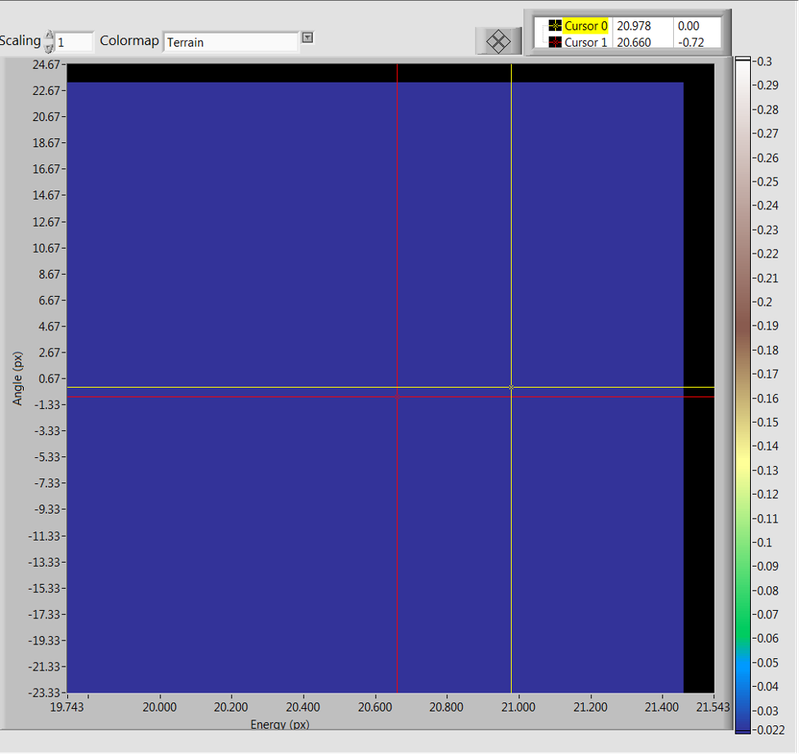
Similar to the "Calibrate Voltages" environment for Scienta software SES, the right side of the GUI shows live updates according to the selected acquisition parameters. Cursor selection works to highlight the area of interest with the yellow crosshairs in the top-right, and the red crosshairs for the bottom-left. The region of interest will be the bounding box created by the yellow/red crosshairs.

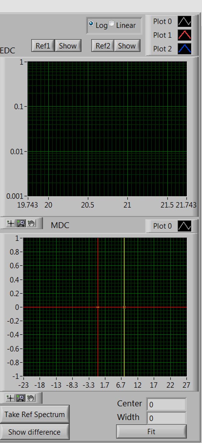
Also shown is the energy-distribution curve (EDC), and the momentum-distribution curve (MDC) also defined by the same bounding box with yellow and red crosshairs.

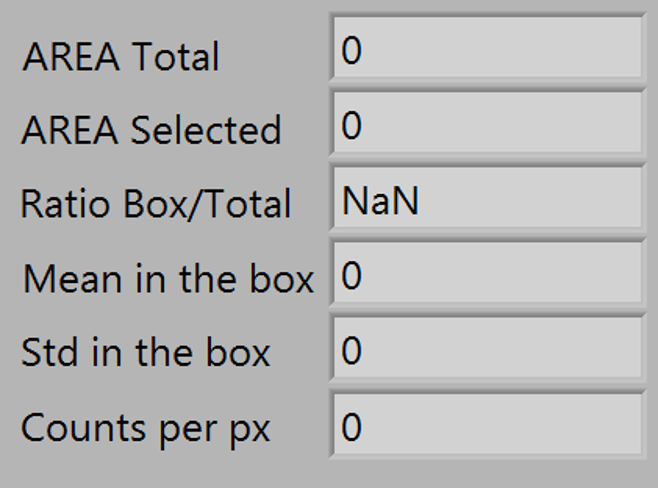
The total count rate (AREA Total), the selected area count rate defined by the yellow and red crosshairs (AREA Selected) are also shown in the lower left area of the GUI. The 'AREA Total' value should be kept below one-to-two million counts (1,000,000 - 2,000,000) to prevent damage to the analyzer micro-channel plate (MCP) detector.

In pursuit of higher statistics, one will often acquire many copies of the image. You can set how many you want by changing the right-side number in the figure below (shown as 1000).

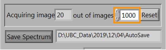
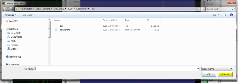
Clicking the 'Reset' button will reset the 'Acquiring image' count back to one. If you desire to save the image being acquired, click on the 'Save Spectrum' button. Once the 'Acquiring image' counter reaches the requested number, a File Save Dialogue window will open, where you can choose the destination location for the file. By default, the file is saved to a folder with the current date. The autosave directory is indicated in the text box to the right of this button.

NOTE: the 'Save Spectrum' will automatically engage for longer acquisitions, in case the user forgets to click the 'Save Spectrum' button. Also it is helpful to un-click the 'Save Spectrum' button when changing the number of total images to a low value, as you will get the File Save Dialogue repeatedly appearing every time the images are acquired.

TROUBLESHOOTING: if you choose to 'Cancel' a save operation, this will cause LabVIEW to pop up an error message.

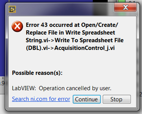
Instead of clicking on 'Stop', choose 'Continue' which will give you the chance to save the file again. Go for this option, and just save the useless data. It will save the LabVIEW program from crashing. If you do click the 'Stop' button, the acquisition program will crash, sending you back to the main LabVIEW window. Note that if you press the 'Run' button again (white arrow), things will not work properly, as communication ports have not been closed during the crash. To recover from this scenario, click the 'Run' button, select the correct pass energy, now click on the 'Finalize' tab, and respond 'Yes' to the pop-up dialogue. Now you will be able to 'Run' the program again as the communication ports have been reset. You know that things are working again when the live Camera View image shows counts. This procedure holds in general for whenever LabVIEW exits unexpectedly.

To do a Fermi surface measurement first define the measurement parameters you will use on the 'Parameters' tab in the acquisition GUI. During the setup of these scan parameters, the program continues to acquire images as defined under this tab.

NOTE: If the 'Dwell Time (ms)' parameter is large, new input in the 'Acquire FS' tab becomes delayed by this amount of time. For example, if the 'Dwell Time (ms)' is set to 10 seconds (10,000 ms), this means that mouse clicks will take 10 seconds to register within LabVIEW.

The most efficient way to set up scan parameters for Fermi surfaces is to first set all the required parameters you will use on the 'Parameters' tab, except for the 'Dwell Time (ms)' parameter. Then select the 'Acquire FS' tab in the main LabVIEW acquisition window:

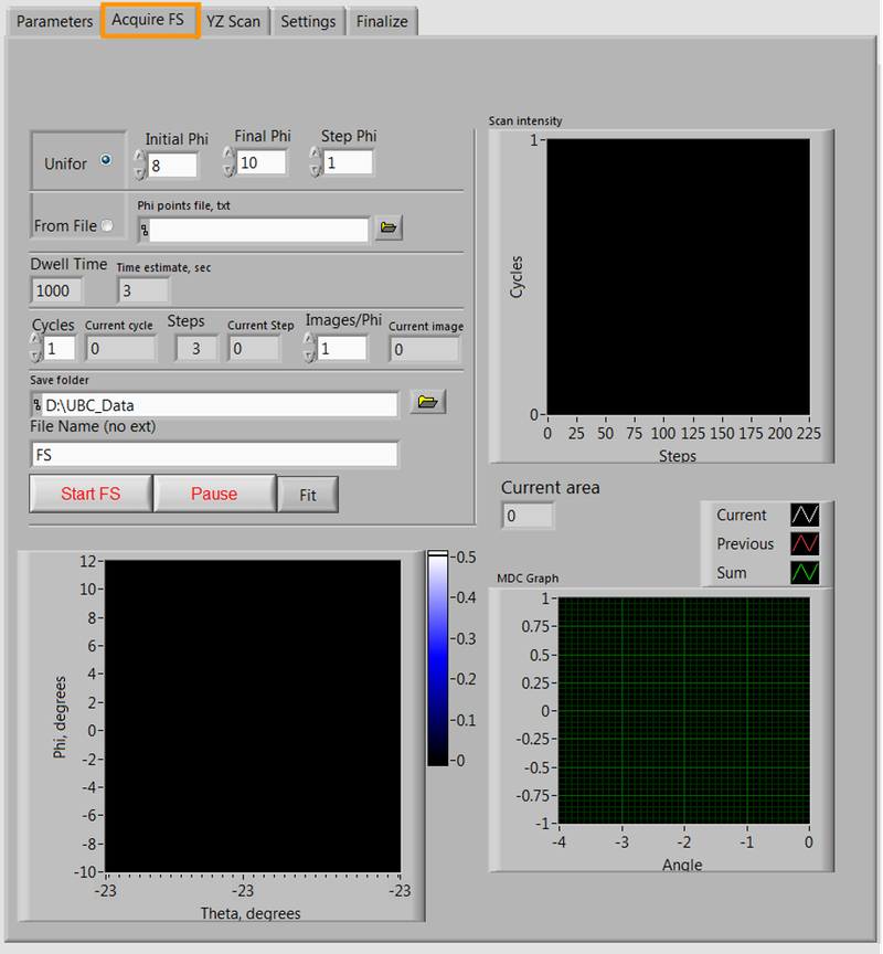
The 'Initial Phi', 'Final Phi', and 'Step Phi' define the rotation about the sample's horizontal axis. Select a Phi range and step size as needed. In the image shown below the scan will go from 8º to 10º in steps of 1º. If you need to define an irregular set of angles, you can load a text file with the angles to measure. Select the radio button 'From File' to enable this functionality. The format for the text file is a 1-column list with each new angle (degrees) entered as a number on a new row.

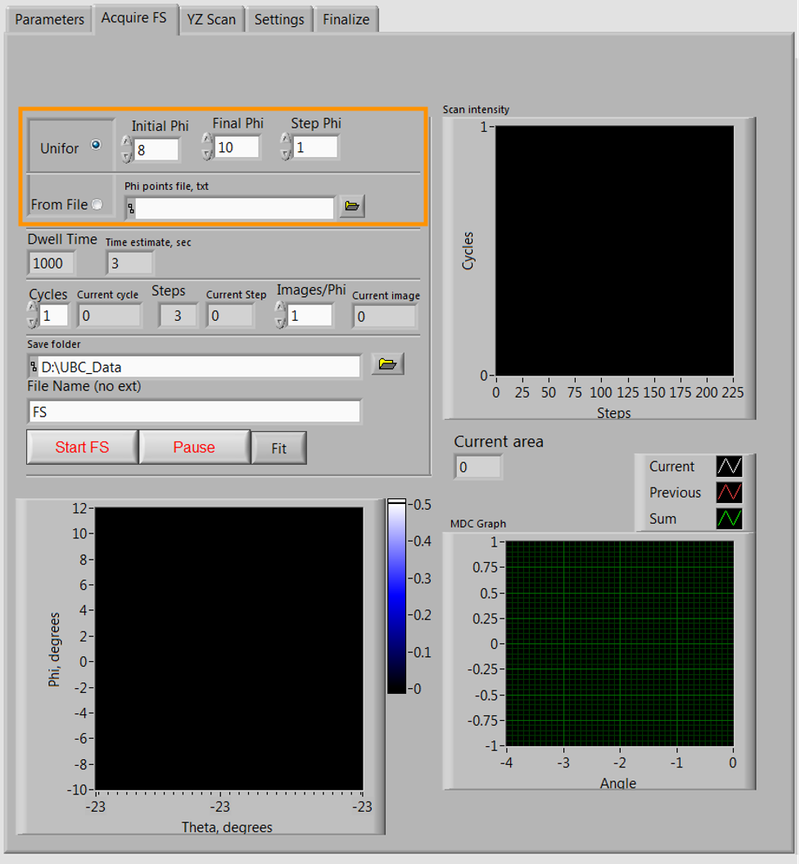
Beside the 'Dwell Time' indicator, you are provided with an estimated total time for your Fermi surface scan in seconds. The number of cycles (iterations) of the Fermi surface you would like to acquire, can also be specified. This is useful for averaging and better statistics. The raw data for each cycle is saved separately to ensure that if perchance there happens to be a storage ring trip, at least some of the data will be useful.

The remaining parameter to define is the 'Images/Phi' value. This option defines how many images are averaged according to the specified 'Dwell Time'. You can reach comparable results two ways, with minimal differences between them. For example having a 'Dwell Time' of 1000 ms and using 10 for the value under 'Images/Phi', is similar to having a 'Dwell Time' of 5000 ms, and selecting 2 'Images/Phi'. There is slightly longer readout overhead with using multiple images versus just having a longer 'Dwell Time' value.

NOTE: a balance between the number of cycles and 'Dwell Time' per Phi angle is important, as running too many cycles versus acquiring more 'Images/Phi' (or increasing the 'Dwell Time') will result in extra dead time due to additional movements between each step that the sample manipulator will need to do. This can be significant over the course of longer scans.

You also need to specify the location to save the data files under the 'Save Folder' area:

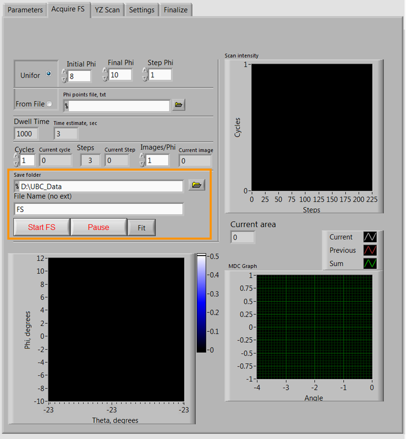
Ensure the correct folder is selected and the file name heading can also be specified here (as shown in the image the filenames will start with 'FS').

Once all parameters are set, go back to the parameters tab and change the 'Dwell Time (ms)' to the value you want, select 'Acquire FS' again and then click the 'Start FS' button to begin the data acquisition.

NOTE: Before clicking 'Start FS' double-check the following two items: (1) ensure the 'Dwell Time (ms)' is the correct value (2) that the energy region of interest is selected with the red/yellow crosshairs - this will ensure the graphs in the GUI show something meaningful and informative while the scan is running.